
The Data Warehouse Setup No One Taught You
Storage is cheap. Your time is not.


Running and using a data warehouse can suck. There are pitfalls. It doesn’t have to be so hard. In fact, it can be so ridiculously easy that you’d be surprised people are paying you so much to do your data engineering job. My name is Sahar. I’m an old coworker of Zach’s from Facebook. This is our story. (Part two is here)
Data engineering can actually be easy, fast, and resilient! All you have to embrace is a simple concept: Date-stamping all your data.
Why isn’t this the norm? Because – even in 2025 — , institutions haven’t really understood the implications that STORAGE IS CHEAP! (And your data team’s time is expensive).
Datestamping solves so many problems. But you won’t find it in a standard textbook. They’ll teach you “slowly changing dimensions Type 2” when the real answer is simpler and more powerful. You will find the answer in Maxime Beauchemin’s seminal article on functional data engineering. Here’s the thing – I love Max, but that article is not helpful to the majority of people who could learn from it.
What if I told you:
We can have resilient pipelines.
We can master changes to data over time.
We can use One Weird Trick to marry the benefits of order and structure with the benefits of chaos and exploration.
That’s where this article comes in. It’s been 7 years in the making – all the stuff that you should know, but no one bothered to tell you yet. (At least, in plain english – sorry Max!)
Part One: How to set up a simple warehouse (and which small bits of jargon actually matter)
Part Two: Date-stamping. Understand this and everyone’s life will become easier, happier, and 90% more bug-free.
Part Three: Plugging metrics into AB testing. Warehousing enables experimentation. Experimentation enables business velocity.
Part Four: The limits of metrics and KPIs. It can be so captivating to chase short-term metrics to long-term doom.
I’ll show you a practical intro to scalable analytics warehousing, where date stamps are the organizing principle, not an afterthought. In plain language, not tied to any specific tool, and useful to you today Meta used this architecture even back in the early 2010s. It worked with Hive metastore. It still works with Iceberg, Delta, and Hudi.
But first, to understand why all this matters, you need some context about how warehouses work. Then I’ll show you the magic.
Sponsorship
Cut Code Review Time & Bugs in Half

Code reviews are critical but time-consuming. CodeRabbit acts as your AI co-pilot, providing instant Code review comments and potential impacts of every pull request.
Beyond just flagging issues, CodeRabbit provides one-click fix suggestions and lets you define custom code quality rules using AST Grep patterns, catching subtle issues that traditional static analysis tools might miss.
CodeRabbit has so far reviewed more than 10 million PRs, installed on 1 million repositories, and used by 70 thousand Open-source projects. CodeRabbit is free for all open-source repo’s.
Part one — A Simple Explanation of Modern Data Warehousing
Our goals and our context
We are here to build a system that gets all company data, tidily, in one place. That allows us to make dashboards that executives and managers look at, charts and tools that analysts and product managers can use to do deep dives, alerts on anomalies, and a breadth of linked data that allows data scientists and researchers to look for magic or product insights. The basic building blocks are tables, and the pipelines that create and maintain them.
Sidebar: DB vs Data lake? OLTP vs OLAP? Production vs warehouse? Here’s what you need to know.
A basic point about a data warehouse (or lake, or pond, or whatever trendy buzzword people use today) is that it is not production. It must be a separate system from “the databases we use to power the product”.
Both are “databases”, both have “data”, including “tables” that might be similar or mirrored – but the similarity should end there.
Your production database is meant to be fast, serve your product and users. It is optimized for code to read and write.
Your warehouse is meant to be human-usable, and serve people inside the business. It is optimized for breadth, for use by human analysts, and to have historical records.
Put it this way – your ecommerce webapp needs to look up an item’s price and return it as fast as possible. Your warehouse needs to look up an item from a year ago, and look at how the price changed over the course of months. The database powering the webapp won’t even store the information, much less make it easy to compute. Meanwhile if you run a particularly difficult query, you don’t want your webapp to slow down.
So – split them. (You might hear people talking about OLTP vs OLAP – it’s just this distinction. Ignore the confusing terminology. Here’s a deep dive into the two types of OLAP data model (Kimball and One Big Table) )
So, we want a warehouse. Ideally, it should:
Be separate from our production databases
Collect all data that is useful to the company
Have tables that make queries easy
Be correct – with accurate, trusted, information
Be reasonably up to date – with perhaps a daily lag, rather than a weekly or monthly one
Power charts and interactive tools, while also being useful for automatic and local queries
This used to be difficult! (It is not anymore!) There was a tradeoff between “big enough to have all the data we need” and “give answers fast enough to be useful”. A lot of hard work was put into reconciling those two needs.
Since circa 2015 or so, this pretty much no longer a problem. Presto/Trino, Spark, and hosted databases (BigQuery, Snowflake, the AWS offerings) and other tools allow you to have arbitrarily huge data, accessed quickly. We live in a golden age.
Sidebar: At my old school…
At Meta, they used HDFS and Hive to power their data lake and MySQL to power production. Once a day they took a “snapshot” of production with a corresponding date stamp and moved the data from MySQL to Hive.
In a world where storage is cheap, access to data can be measured in seconds rather than minutes or hours, and data is overflowing, the bottleneck is engineering time and conceptual complexity. Solving that bottleneck allows us to break with annoyingly fiddly past best practices. That’s what I’m here to talk about.
A basic setup
Imagine your warehouse as a giant box, holding many, many tables. Think of data flowing downhill through it.
At the top: raw copies from production databases, marketing APIs, payment processors, whatever.
At the bottom: clean, trusted tables that analysts actually query.
In between: pipelines that flow data from table to table.
[Raw Input Tables]
├─ users_production
├─ events_raw
├─ transactions_raw [Pipelines]
└─ ... ↓

     Clean → Join → Enrich

                 ↓

[Clean Output Tables]
├─ dim_users
├─ fct_events
└─ grp_daily_revenue
How do we get from raw input to clean tables? Pipelines. (See buzzwords like ETL, ELT? Ignore the froth – replace with “pipelines” and move on).
Pipelines are the #1 tool of data engineering. At their most basic form, they’re pieces of code that take in one or more input tables, do something to the data, and output a different table.
What language do you write pipelines in? Like it or not, the lingua franca of editing large-scale data is SQL. The lingua franca of accessing large scale data is SQL. SQL is a constrained enough language that it can parallelize easily. The tools that invisibly translate your simple snippets into complex mechanisms to grab data from different machines, transform it, join it, etc – they not only are literally set up with SQL in mind, they figuratively cannot do the same for python, java, etc. Why? Because a traditional programming language gives you too much flexibility -- there’s no guarantee that your imperative code can be parallelized nicely.
Sidebar: When non-SQL makes sense (or doesn’t)
If you’re ingesting data from the outside world (calling APIs, reading streams, and so on), then python, javascript, etc could make sense. But once data is in the warehouse, beware anything that isn’t SQL – it’s likely unnecessary, and almost certainly going to be much slower than everything else.
Your tooling might offer a way to “backdoor” a bit of code (e.g. “write some java code that calls an API and then writes the resultant variable to a column”). Think twice before you use it. Often, it’s easier and faster to import a new dataset into your warehouse so that you can recreate with SQL joins what you would have done using an imperative language.
You may be tempted to transform or analyze data in R, pandas, or whatnot – that’s fine, but you do that by interactively reading from the warehouse. Rule of thumb: if you’re writing between tables in a warehouse – SQL. Into a warehouse – you probably need some glue code somewhere. Out of a warehouse – that’s on you.
So here’s the simple setup:
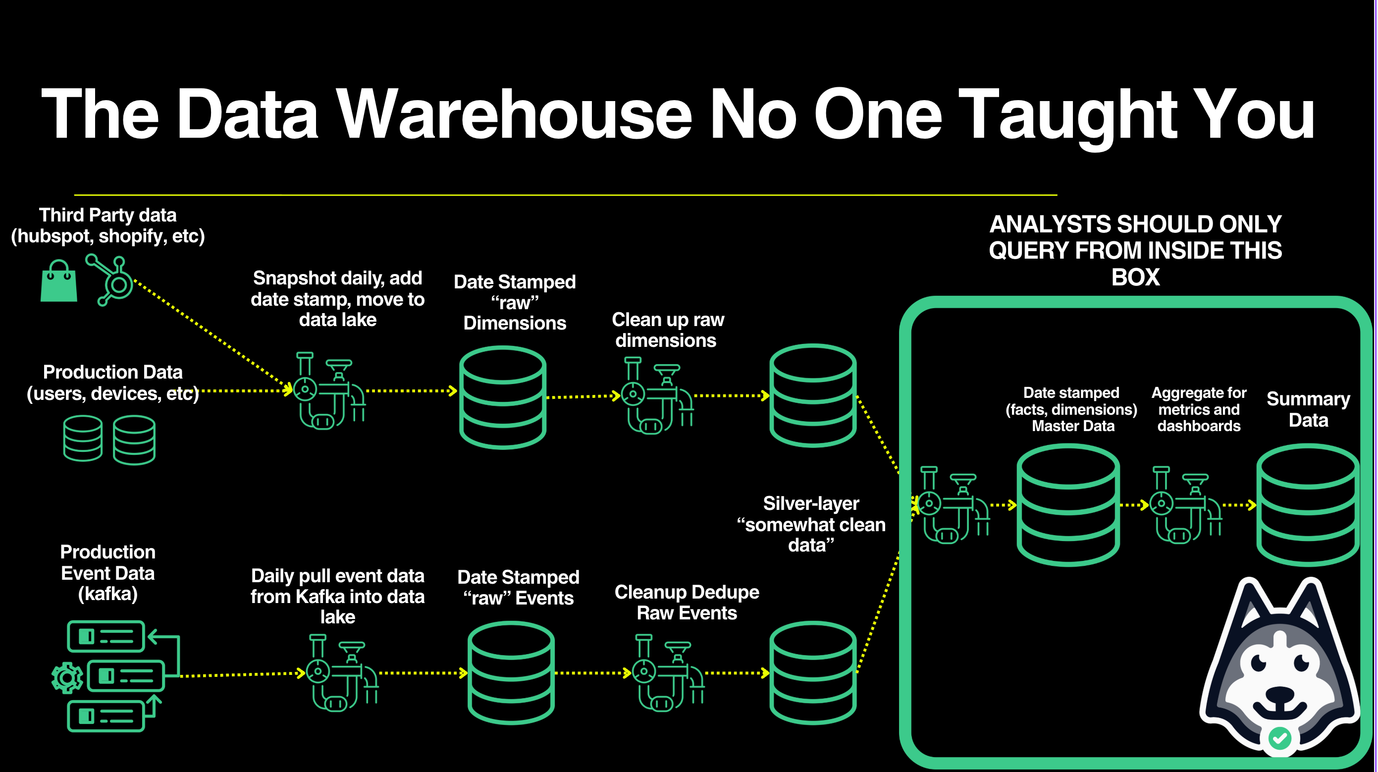
Then, set up a system of pipelines to this, every day, as soon as the upstream data is ready:
As each of these input tables gets the latest dump of data from outside: take that latest day’s data, deduplicate, clean it up a bit, rename the columns, and cascade it to a nicer, cleaner version of that table. (this is your silver tier data in medallion architecture)
Then, from that nicer input table, perform a host of transformations, joins, etc to write to other downstream tables. (this is your master data)
Master data is highly trusted which makes building metrics and powering dashboards easy!1
Every day, new data comes in, and your pipeline setup cascades new information in a host of tables downstream of it. That’s the setup.
A well-ordered table structure
Okay, so to review: the basic useful item in a warehouse is a table. Tables are created (and filled up by) pipelines.
“Great, great,” you might say – “but which tables do I build?”
For the sake of example, let’s imagine our product is a social network. But this typology should work just as well for whichever business you are in – from b2b saas to ecommerce to astrophysics.
From the perspective of the data warehouse as a product, there are only three kinds of tables: input tables (copied from outside), staging tables (used by pipelines and machines), and output tables – also known as user-facing tables.
Output tables (in fact, almost all tables) really only have three types:
Tables where each row corresponds to a noun. (E.g. “user”, or even “post” or “comment”). When done right, these are called dimension tables. Prefix their names with dim_
Tables where each row corresponds to an action. Think of them as fancier versions of logs. (E.g. “user X wrote post Y at time Z”). When done right, these are called fact tables. Prefix their names with fct_
Everything else. Often these will be summary tables. (e.g. “number of users who made at least 1 post, per country, per day). If you’re proud of these, prefix them with sum_ or agg_.
Sidebar: more on naming
YMMV, but I generally don’t prefix input tables. Input tables should be an exact copy of the table you’re importing from outside the warehouse. Changing names breaks that – and an unprefixed table name is a good sign that the table cannot be trusted.
Staging and temporary tables are prefixed with stg_ or tmp_.
Let’s talk more about dimension and fact tables, since they’re the core part of any clean warehouse.
Dimension tables are the clean, user-friendly, mature form of noun tables.
Despite being focused on nouns (say, users), they can also roll up useful verby information (leveraging cumulative table design)
For instance, a dim_users table might both include stuff like: user id, date created, datetime last seen, number of friends, name; AND more aggregate “verby” information like: total number of posts written, comments made in the last 7 days, number of days active in the last month, number of views yesterday.
If a data analyst might consistently want that data – maybe add it to the table! Your small code tweak will save them hours of waiting a week.2
(Now, what’s to stop the table from being unusably wide? Say, with 500+ columns? Well, that’s mostly an internal culture problem, and somewhat a tooling problem. You could imagine, say, dim_user getting too large, so the more extraneous information is in a dim_user_extras table, to be joined in when necessary. Or using complex data types to reduce the number of columns)
Fact tables are the clean, user-friendly, mature form of logs (or actions or verb tables).
Despite being verb focused, fact tables contains noun information. (Zach chimes in: here’s a free 4 hour course on everything you need to know about fact tables)
Unlike a plain log, which will be terse, they can also be enriched with data that might probably live in a dim table.
The essence of a good fact table is providing all the necessary context to do analysis of the event in question.
A fact table, fundamentally, helps you understand: “Thing X happened at time Y. And here’s a bunch of context Z that you might enjoy”.
So a log containing “User Z made comment Xa on post Xb at time Y” could turn into a fct_comment table, with fields like: commenter id, comment id, post id, time, time at commenter timezone, comment text, post text, userid of owner of post, time zone of owner of parent post. Some of these fields are strictly speaking unnecessary – you could in theory do some joins to grab the post text, or the comment text, or time zone of the owner of the parent post. But they’re useful to have handy for your users, so why not save them time and grab them anyway.
Q: Wait – so if dim tables also have verb data, and fact tables also have noun data, what’s the difference?
A: Glad you asked. Here’s what it boils down to – is there one row per noun in the table? Dim. One row per “a thing happened?” Fact. That’s it. You’re welcome.
Here, as in so much, we are spending space freely. We are duplicating data. We are also doing a macro form of caching – rather than forcing users to join or group data on the fly, we have pipelines do it ahead of time.
Compute is cheap, storage is cheap. Staff time is not. We want analysis to be fluid and low latency – both technically in terms of compute, and in terms of mental overhead.
Q: Wait! What about data stamps? Where’s the magic? You promised magic.
A: Patience, young grasshopper. Part of enlightenment is the journey. Part of understanding the magic is understanding what it builds on. And – hey – would YOU read a huge blog post all at once? Or would you prefer to read it in chunks. Yeah, you with your Tiktok problem and inability to focus. I’m surprised you even made this far.
Stay tuned for part two where we:
Show you how to make warehousing dirt easy
Behold the glory of date stamping
Through better data quality
Bug fixes are easy now
You get a time machine for free
Explore the dream of functional data engineering (what is that weird phrase?)
Throw SCD-2 and other outdated “solutions” to the dustbin of history
Make sure to follow Sahar’s blog to understand growth and what comes next, both personally and for your business! Sahar is currently open to work, he is interested in DevRel and engineering leadership roles in New York City.
For instance, join the data from your sales and marketing platforms to create a “customer” table. Or join various production tables to create a “user” table. Could you then combine “customer” and “user” to create a bigger table? You might add pipeline steps to create easy tables for analysts to use: “daily revenue grouped by country”, etc.
Here’s another key insight: data processing done while everyone is asleep is much better than data querying done while people are on the clock and fighting a deadline
Can't wait for part2!!
This is probably the most crucial addendum to the standard dimensional modeling books. There is a timeless core there and then a ton of now pointless trivia for creating brittle logic to deal with 2008 era RDBMS storage and compute constraints. Can’t recommend this and the followup post enough to anyone building or using analytics pipelines.